
Step 1 – Collect the Data
To develop the naive Bayes classifier, we will use data adapted from the SMS Spam Collection at http://www.dt.fee.unicamp.br/~tiago/smsspamcollection/.
This dataset includes the text of SMS messages along with a label indicating whether the message is unwanted. Junk messages are labelled spam, while legitimate messages are labelled ham.
The following is a sample of ‘ham’ messages:
Better. Made up for Friday and stuffed myself like a pig yesterday. Now I feel
bleh. But at least its not writhing pain kind of bleh.
If he started searching he will get job in few days. He have great potential
and talent.
I got another job! The one at the hospital doing data analysis or something, starts
on monday! Not sure when my thesis will got finished
The following is a sample ‘spam’ messages:
Congratulations ur awarded 500 of CD vouchers or 125gift guaranteed & Free
entry 2 100 wkly draw txt MUSIC to 87066
December only! Had your mobile 11mths+? You are entitled to update to the latest
colour camera mobile for Free! Call The Mobile Update Co FREE on 08002986906
Valentines Day Special! Win over £1000 in our quiz and take your partner on the
trip of a lifetime! Send GO to 83600 now. 150p/msg rcvd.
Looking at the preceding sample messages, there are some distinguishing characteristics about spam such as the word ‘free’. Days of the week on the other hand are mentioned in the ham messages but not the Spam ones.
Our naive Bayes classifier will take advantage of such patterns in the word frequency to determine whether the SMS messages seem to better fit the profile of spam or ham. While it's not inconceivable that the word "free" would appear outside of a spam SMS, a legitimate message is likely to provide additional words providing context. For instance, a ham message might state "are you free on Sunday?", whereas a spam message might use the phrase "free ringtones." The classifier will compute the probability of spam and ham given the evidence provided by all the words in the message.
Step 2 – Exploring and preparing the data
Text data are challenging to prepare because it is necessary to transform the words and sentences into a form that a computer can understand. We will transform our data into a representation known as bag-of-words, which ignores the order that words appear in and simply provides a variable indicating whether the word appears at all.
Access to this data will be on the Packt Publishing website where it should be downloaded to your R directory /folder. It will likely be necessary to make a purchase first in this particular example, especially as the original data set has been modified to suit the R language. We will assign the file to a variable called sms_raw.
sms_raw <- read.csv("sms_spam.csv", stringsAsFactors = FALSE)
We look at the structure and find that there are 5559 objects and two features, namely type (ham and spam) and text which contains the unstructured SMS messages.

The type variable is currently a character vector. Since this is a categorical variable, it would be better to convert it to a factor, as shown in the following code:
sms_raw$type <- factor(sms_raw$type)
Examining the type variable with the str() and table() functions, we see that the variable has now been appropriately recoded as a factor. Additionally, we see that 747 (or about 13 percent) of SMS messages in our data were labeled spam, while the remainder were labeled ham:
> str(sms_raw$type)
Factor w/ 2 levels "ham","spam": 1 1 1 2 2 1 1 1 2 1 ...
> table(sms_raw$type)
ham spam
4812 747
Data preparation – Processing text data for analysis
We need a powerful set of tools to process text data.
SMS messages are strings of text composed of words, spaces, numbers, and punctuation. Handling this type of complex data takes a large amount of thought and effort. One needs to consider how to remove numbers, punctuation, handle uninteresting words such as and, but, and or, and how to break apart sentences into individual words. Thankfully, this functionality has been provided by members of the R community in a text mining package titled tm.
The tm text mining package can be installed via the install.packages("tm")command and loaded with library(tm).
The first step in processing text data involves creating a corpus, which refers to a collection of text documents. In our project, a text document refers to a single SMS message. We'll build a corpus containing the SMS messages in the training data using the following command:
> sms_corpus <- Corpus(VectorSource(sms_raw$text))
This command uses two functions. First, the Corpus() function creates an R object to store text documents. This function takes a parameter specifying the format of the text documents to be loaded. Since we have already read the SMS messages and stored them in an R vector, we specify VectorSource(), which tells Corpus() to use the messages in the vector sms_train$text. The Corpus() function stores the result in an object named sms_corpus.
If we print() the corpus we just created, we will see that it contains documents for each of the 5,559 SMS messages in the training data:
> print(sms_corpus)
A corpus with 5559 text documents
To look at the contents of the corpus, we can use the inspect() function. By combining this with methods for accessing vectors, we can view specific SMS messages. The following command will view the first, second, and third SMS messages:
> inspect(sms_corpus[1:3])
[[1]]
Hope you are having a good week. Just checking in
[[2]]
K..give back my thanks.
[[3]]
Am also doing in cbe only. But have to pay.
The corpus now contains the raw text of 5,559 text messages. Before splitting the text into words, we will need to perform some common cleaning steps in order to remove punctuation and other characters that may clutter the result. For example, we would like to count hello!, HELLO..., and Hello as instances of the word hello
The function tm_map() provides a method for transforming (that is, mapping) a tm corpus. We will use this to clean up our corpus using a series of transformation functions, and save the result in a new object called corpus_clean.
First, we will convert all of the SMS messages to lowercase and remove any numbers:
> corpus_clean <- tm_map(sms_corpus, tolower)
> corpus_clean <- tm_map(corpus_clean, removeNumbers)
A common practice when analyzing text data is to remove filler words such as to, and, but, and or. These are known as stop words. Rather than define a list of stop words ourselves, we will use the stopwords() function provided by the tm package. It contains a set of numerous stop words. To see them all, type stopwords() at the command line. As we did before, we'll use the tm_map() function to apply this function to the data:
corpus_clean <- tm_map(corpus_clean, removeWords, stopwords())
We'll also remove punctuation:
corpus_clean <- tm_map(corpus_clean, removePunctuation)
Now that we have removed numbers, stop words, and punctuation, the text messages are left with blank spaces where these characters used to be. The last step then is to remove additional whitespace, leaving only a single space between words.
Now that we have removed numbers, stop words, and punctuation, the text messages are left with blank spaces where these characters used to be. The last step then is to remove additional whitespace, leaving only a single space between words.
> corpus_clean <- tm_map(corpus_clean, stripWhitespace)
The following table shows the first three messages in SMS corpus before and after the cleaning process. The messages have been limited to the most interesting words and punctuation and capitalization have been removed:

When the data set is finally to one’s liking the final step is to split the messages into individual components through a process called tokenization. A token is a single element of a text string; in this case, the tokens are words.
The tm package provides functionality to tokenize the SMS message corpus. The DocumentTermMatrix() function will take a corpus and create a data structure called a sparse matrix, in which the rows of the matrix indicate documents (that is, SMS messages) and the columns indicate terms (that is, words). Each cell in the matrix stores a number indicating a count of the times the word indicated by the column appears in the document indicated by the row. The following screenshot illustrates a small portion of the document term matrix for the SMS corpus, as the complete matrix has 5,559 rows and over 7,000 columns:

The fact that each cell in the table is zero implies that none of the words listed at the top of the columns appears in any of the first five messages in the corpus. This highlights the reason why this data structure is called a sparse matrix; the vast majority of cells in the matrix are filled with zeros. Although each message contains some words, the probability of any specific word appearing in a given message is small.
Creating a sparse matrix given a tm corpus involves a single command:
> sms_dtm <- DocumentTermMatrix(corpus_clean)
This will tokenize the corpus and return the sparse matrix with the name sms_dtm. From here, we'll be able to perform analyses involving word frequency.
However as you can see from the output in R, there was an error. The suggestion presented on StackOverFlow, below appears to have fixed the error.

The lines were re-entered starting with the command: > corpus_clean <- tm_map(corpus_clean, PlainTextDocument) and this was run.

Data preparation – Creating Training and Data Sets
Since our data have been prepared for analysis, we now need to split the data into a training dataset and test dataset so that the spam classifier can be evaluated on data it had not seen previously. We'll divide the data into two portions: 75 percent for training and 25 percent for testing. Since the SMS messages are sorted in a random order, we can simply take the first 4,169 for training and leave the remaining 1,390 for testing.
We'll begin by splitting the raw data frame:
> sms_raw_train <- sms_raw[1:4169, ]
> sms_raw_test <- sms_raw[4170:5559, ]
Then the document-term matrix:
> sms_dtm_train <- sms_dtm[1:4169, ]
> sms_dtm_test <- sms_dtm[4170:5559, ]
And finally, the corpus:
> sms_corpus_train <- corpus_clean[1:4169]
> sms_corpus_test <- corpus_clean[4170:5559]
To confirm that the subsets are representative of the complete set of SMS data, let's compare the proportion of spam in the training and test data frames:
> prop.table(table(sms_raw_train$type))
ham spam
0.8647158 0.1352842
> prop.table(table(sms_raw_test$type))
ham spam
0.8683453 0.1316547
Both the training data and test data contain about 13 percent spam. This suggests that the spam messages were divided evenly between the two datasets.
Visualizing Text Data – Word Clouds
A word cloud is a way to visually depict the frequency at which words appear in text data. The cloud is made up of words scattered somewhat randomly around the figure. Words appearing more often in the text are shown in a larger font, while less common terms are shown in smaller fonts. This type of figure has grown in popularity recently since it provides a way to observe trending topics on social media websites.
The wordcloud package provides a simple R function to create this type of diagram. We'll use it to visualize the types of words in SMS messages. Comparing the word clouds for spam and ham messages will help us gauge whether our naive Bayes spam filter is likely to be successful. If you haven't already done so, install the package by typing install.packages("wordcloud") and load the package by typing library(wordcloud) at the R command line.
A word cloud can be created directly from a tm corpus object using the syntax:
> wordcloud(sms_corpus_train, min.freq = 40, random.order = FALSE)
This will create a word cloud from sms_corpus_train corpus. Since we specified random.order = FALSE, the cloud will be arranged in non-random order, with the higher-frequency words placed closer to the center. If we do not specify random.order, the cloud would be arranged randomly by default. The min.freq parameter specifies the number of times a word must appear in the corpus before it will be displayed in the cloud. A general rule is to begin by setting min.freq to a number roughly 10 percent of the number of documents in the corpus; in this case 10 percent is about 40. Therefore, words in the cloud must appear in at least 40 SMS messages.
The instructions and resulting ‘wordcloud’ can be seen below:


Another interesting visualization involves comparing the clouds for SMS spam and ham. Since we did not construct separate corpora for spam and ham, this is an appropriate time to note a very helpful feature of the wordcloud() function. Given raw text, it will automatically apply text transformation processes before building a corpus and displaying the cloud. Let's use R's subset() function to take a subset of the sms_raw_train data by SMS type. First, we'll create a subset where type is equal to spam:
> spam <- subset(sms_raw_train, type == "spam")
Next, we'll do the same thing for the ham subset:
> ham <- subset(sms_raw_train, type == "ham")
We now have two data frames, spam and ham, each with a text feature containing
the raw text strings for SMS messages. Creating word clouds is as simple as before.
This time, we'll use the max.words parameter to look at the 40 most common words
in each of the two sets. The scale parameter allows us to adjust the maximum and
minimum font size for words in the cloud. Feel free to adjust these parameters as
you see fit. This is illustrated in the following code:
> wordcloud(spam$text, max.words = 40, scale = c(3, 0.5))
> wordcloud(ham$text, max.words = 40, scale = c(3, 0.5))
The resulting word clouds are shown in the following diagram. Do you have a hunch
which one is the spam cloud and which represents ham?

If you hadn't already guessed, the spam cloud is on the left. Spam SMS messages include words such as urgent, free, mobile, call, claim, and stop; these terms do not appear in the ham cloud at all. Instead, ham messages use words such as can, sorry, need, and time. These stark differences suggest that our naive Bayes model will have some strong key words to differentiate between the classes.
Data preparation – creating indicator features for frequent words
The final step in the data preparation process is to transform the sparse matrix into a data structure that can be used to train a naive Bayes classifier. Currently, the sparse matrix includes over 7,000 features a feature for every word that appears in at least one SMS message. It's unlikely that all of these are useful for classification. To reduce the number of features, we will eliminate any words that appear in less than five SMS messages, or less than about 0.1 percent of records in the training data. Finding frequent words requires use of the findFreqTerms() function in the tm package. This function takes a document term matrix and returns a character vector containing the words appearing at least a specified number of times. For instance, the following command will display a character vector of the words appearing at least 5 times in the sms_dtm_train matrix:
> findFreqTerms(sms_dtm_train, 5)
To save this list of frequent terms for use later, we'll use the Dictionary() function:
> sms_dict <- Dictionary(findFreqTerms(sms_dtm_train, 5))
Following this attempt the following error occurred:
The Dictionary function has been deprecated as seen in this StackOverFlow solution.
Various attempts were tried to overcome this but in the end we created a dummy function called Dictionary to try and get around this. No errors appeared to occur with this solution.
In previous versions of ‘tm’ function it was intended that a dictionary be a data structure allowing us to specify which words should appear in a document term matrix. To limit our training and test matrixes to only the words in the preceding dictionary, one would use the following commands:
> sms_train <- DocumentTermMatrix(sms_corpus_train,
list(dictionary = sms_dict))
> sms_test <- DocumentTermMatrix(sms_corpus_test,
list(dictionary = sms_dict))
The training and test data now includes roughly 1,200 features corresponding only to words appearing in at least five messages. The naive Bayes classifier is typically trained on data with categorical features. This poses a problem since the cells in the sparse matrix indicate a count of the times a word appears in a message. We should change this to a factor variable that simply indicates yes or no depending on whether the word appears at all.
The following code defines a convert_counts() function to convert counts to factors:
> convert_counts <- function(x) {
x <- ifelse(x > 0, 1, 0)
x <- factor(x, levels = c(0, 1), labels = c(""No"", ""Yes""))
return(x)
}
By now, some of the pieces of the preceding function should look familiar. The first line defines the function. The statement ifelse(x > 0, 1, 0) will transform the values in x so that if the value is greater than 0, then it will be replaced with 1, otherwise it will remain at 0. The factor command simply transforms the 1 and 0 values to a factor with labels No and Yes. Finally, the newly-transformed vector x is returned. Now, we just need to apply convert_counts to each of the columns in our sparse matrix. You may be able to guess the R function can do exactly that; it's stated in the preceding sentence. The function is simply called apply().
The apply() function allows a function to be used on each of the rows or columns in a matrix. It uses a MARGIN parameter to specify either rows or columns. Here, we'll use MARGIN = 2 since we're interested in the columns (MARGIN = 1 is used for rows). The full commands to convert the training and test matrixes are as follows:
> sms_train <- apply(sms_train, MARGIN = 2, convert_counts)
> sms_test <- apply(sms_test, MARGIN = 2, convert_counts)
The result will be two matrixes, each with factor type columns indicating Yes or No
for whether each column's word appears in the messages comprising the rows.
Step 3 – training a model on the data
Now that we have transformed the raw SMS messages into a format that can be represented by a statistical model, it is time to apply the naive Bayes algorithm. The algorithm will use the presence or absence of words to estimate the probability that a given SMS message is spam.
The naive Bayes implementation we will employ is in the e1071 package. This package was developed at the statistics department at the Vienna University of Technology (TU Wien), and includes a variety of functions for machine learning. If you have not done so already, be sure to prepare the package using the commands, install.packages("e1071") and library(e1071) before continuing.
Unlike the kNN algorithm we used for classification in the previous chapter, training a naive Bayes learner and using it for classification occur in separate stages. Still, as shown in the following table, classification is fairly straightforward:
To build our model on the sms_train matrix, we'll use the following command:
sms_classifier <- naiveBayes(sms_train, sms_raw_train$type)
The sms_classifier variable now contains a naïve Bayes classifier object that can be used to make predictions.
Step 4 – evaluating model performance
To evaluate the SMS message classifier, we need to test its predictions on the unseen messages in the test data. Recall that the unseen message features are stored in a matrix named sms_test, while the class labels spam or ham are stored in a vector named type in the sms_raw_test data frame. The classifier that we trained has been named sms_classifier. We will use this to generate predictions, and we will compare the predictions to the true values. The predict() function is used to make the predictions. We will store these in a vector named sms_test_pred:
sms_test_pred <- predict(sms_classifier, sms_test)
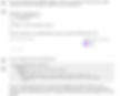
The image below shows Step 3 and Step 4 inputs:

To compare the predicted values to the actual values, we'll use the CrossTable() function in the gmodels package, which we have used previously. This time, we'll add some additional parameters to eliminate unnecessary cell proportions, and usethe dnn parameter (dimension names) to relabel the rows and columns, as shown in the following code:
library(gmodels)
CrossTable(sms_test_pred, sms_raw_test$type,
prop.chisq = FALSE, prop.t = FALSE,
dnn = c('predicted', 'actual'))
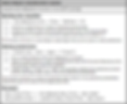
The following output was produced:

Looking at the table, we can see that 4 of 1207 ham messages (0.3 percent) were incorrectly classified as spam, while 32 of 183 spam messages (17.5 percent) were incorrectly classified as ham. Considering the little effort we put into the project, this level of performance seems quite impressive. This case study exemplifies the reason why naive Bayes is the standard for text classification; directly out of the box, it performs surprisingly well.
On the other hand, the four legitimate messages that were incorrectly classified as spam could cause significant problems for the deployment of our filtering algorithm. If the filter caused a person to miss an important text message for an appointment or emergency, they would quickly abandon the product. We should investigate the incorrectly classified SMS messages to see where things went wrong.
Step 5 – improving model performance
You may have noticed that we didn't set a value for the Laplace estimator when training our model. This allows words that appeared in zero spam or zero ham messages to have an indisputable say in the classification process. Just because the word "ringtone" only appeared in spam messages in the training data, it does not mean that every message with that word should be classified as spam.
We'll build a naive Bayes model as before, but this time set laplace = 1:
sms_classifier2 <- naiveBayes(sms_train, sms_raw_train$type, laplace = 1)
Next, we'll make predictions:
sms_test_pred2 <- predict(sms_classifier2, sms_test)
Finally, we'll compare the predicted classes to the actual classifications using
a cross tabulation:
CrossTable(sms_test_pred2, sms_raw_test$type,
prop.chisq = FALSE, prop.t = FALSE, prop.r = FALSE,
dnn = c('predicted', 'actual'))
This results in the following table:

In spite of reducing the number of false positives (ham messages erroneously classified as spam) from four to three, we also reduced the number of false negatives from 32 to 31. Although this seems like a small improvement, we must also be aware of the potential for important messages to be missed if we are too aggressive at filtering spam.
Summary
This algorithm constructs tables of probabilities that are used to estimate the likelihood that new examples belong to various classes. The probabilities are calculated using a formula known as Bayes' theorem, which specifies how dependent events are related.
Although Bayes' theorem can be computationally expensive to process, a simplified version that makes so-called "naive" assumptions about the independence of features is capable of being used with extremely large datasets. The naive Bayes classifier is often used for text classification. To illustrate its effectiveness, we employed naive Bayes on a classification task involving filtering spam SMS messages. Preparing the text data for analysis required the use of specialized R packages for text processing and visualization. Ultimately, the model was able to classify nearly 98 percent of all SMS messages correctly as spam or ham.